Fold the mini-protein, chignolin

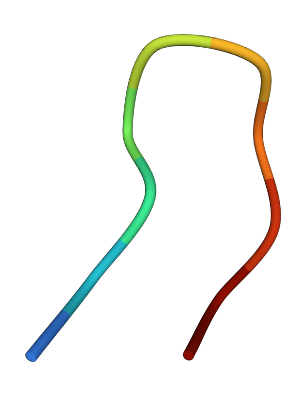
Chignolin is an artificial mini-protein consisting of only 10 amino acid residues. Here we use potential contrasting to learn a coarse-grained force field that can capture the protein’s folding and unfolding

1. Download the all-atom simulation trajectory

An all-atom simulation of chignolin is used as training data. You can follow the link pccg-chignolin to download the all-atom simulation trajectory. Then you should uncompress the downloaded data and move them to the directory WORK_DIR/data. Here WORK_DIR can be any directory and wil be used as the working directory for running commands in the tutorial. In other words, you should change your working directory to WORK_DIR before running following commands. In the direcotry WORK_DIR/data, there should be three files:

• cln025_all_atom.dcd: an all-atom simulation trajectory

• cln025.prmtop: the topology file of chignolin

• cln025_reference.pdb: a folded conformation of chignolin

The all-atom simulation was conducted with implicit solvent and near the folding temperature, so the all-atom simulation trajectory contains both folded and unfolded conformations. You can visualize the trajectory by loading it together with the topology file into softwares such as VMD.

2. Convert the all-atom trajectory into a coarse-grained one

First we need to choose a coarse-grained representation for the force field. Here we choose to represent each amino acid residue with just one particle fixed at the residue’s \(\alpha\) carbon atom postion. With this coarse-grained representation, let us convert the all-atom trajectory into a coarse-grained one, which will be used as training data.

import numpy as np
import matplotlib as mpl
import matplotlib.pyplot as plt
import mdtraj
import os
import scipy
import scipy.optimize as optimize
import scipy.cluster.hierarchy
from scipy.spatial.distance import squareform
import torch
import math
import openmm
import openmm.unit as unit
import openmm.app as ommapp
import time
from sys import exit

#### convert the all atom trajectory into a coarse-grained one
top_aa = mdtraj.load_prmtop('./data/cln025_all_atom.prmtop')
traj_aa = mdtraj.load_dcd('./data/cln025_all_atom.dcd', top_aa, stride = 10)

alpha_carbon_atom_indices = []
for atom in top_aa.atoms:
    if atom.name == 'CA':
        alpha_carbon_atom_indices.append(atom.index)
traj_cg = traj_aa.atom_slice(alpha_carbon_atom_indices)

os.makedirs('./output/', exist_ok = True)
traj_cg.save_dcd('./output/cln025_cg.dcd')

We can visualize the coarse-grained trajectory by projecting conformations into a low dimensional space spanned by collective variables such as the RMSD (root-mean-squared-distance) with respect to the folded conformations.

top_cg = mdtraj.load_psf('./data/cln025_cg.psf')
traj_cg = mdtraj.load_dcd('./output/cln025_cg.dcd', top_cg)

ref_pdb = mdtraj.load_pdb('./data/cln025_reference.pdb')
ref_pdb = ref_pdb.atom_slice(alpha_carbon_atom_indices)
ref_traj = mdtraj.Trajectory(ref_pdb.xyz, topology = top_cg)
rmsd = mdtraj.rmsd(traj_cg, ref_traj)

fig = plt.figure()
fig.clf()
plt.hist(rmsd, bins = 30, density = True, range = (0, 0.8), color = 'C1', label = 'All atom')
plt.legend()
plt.xlabel('RMSD (nm)')
plt.ylabel('Probablity density')
plt.tight_layout()
plt.savefig('./output/rmsd_hist_all_atom.png')
plt.close()

3. Construct a noise distribution and generate noise samples

In potential contrasting, we construct the noise distribution by learning an energy function and use the corresponding Boltzmann distribution as the noise distribution. Here we use an energy function that includes terms for bonds, angles, and dihedrals defined as

\[u_\mathrm{bonded}(b, a, d) = \sum_{i=1}^{L-1} \frac{1}{2}k_i (b_i - b_i^\circ)^2 + \sum_{i=1}^{L-2} S_\mathrm{angle}(a_i; \boldsymbol{c}^a_i) + \sum_{i=1}^{L-3} S_\mathrm{dihedral}(d_i; \boldsymbol{c}^d_i),\]

where \(L = 10\) is the number of residues in the protein, and \(b_i, a_i\), and \(d_i\) represent the \(i\) th bond, angle, and dihedral angle, respectively. A quadratic function is used for energies on bonds. \(k_i\) and \(b_i^\circ\) are the force constant and the equilibrium value for the \(i\) th bond, respectively. Cubic spline functions, \(S_\mathrm{angle}\) and \(S_\mathrm{dihedral}\), are used for energies on angles and dihedral angles. \(\boldsymbol{c}^a_i\) and \(\boldsymbol{c}^d_i\) are spline coefficients for the \(i\) th angle and dihedral angle, respectively.

Because individual energy terms in \(u_\mathrm{bonded}(b, a, d)\) are separable, we can fit their paramters independently such that each energy term will reproduce the marginal distribution of the corresponding internal coordinate. For bond paramters, we can estimate them directly using the mean and the variance of bond length distributions. For angle and dihedral parameters, we use the noise contrastive estimation with uniform distributions as the noise distribution. We note that the unit of energy in \(u_\mathrm{bonded}(b, a, d)\) is \(kT\).

n_atoms = top_cg.n_atoms
bonded_terms = {
    'bond': {'indices': np.array([[i,i+1] for i in range(n_atoms - 1)])},
    'angle': {'indices': np.array([[i,i+1,i+2] for i in range(n_atoms - 2)])},
    'dihedral': {'indices': np.array([[i,i+1,i+2,i+3] for i in range(n_atoms - 3)])}
}

#### fit parameters for bonds
bonded_terms['bond']['b0'] = []
bonded_terms['bond']['kb'] = []
for i in range(bonded_terms['bond']['indices'].shape[0]):
    atom_pair = bonded_terms['bond']['indices'][i]
    dist = mdtraj.compute_distances(traj_cg, atom_pairs = [atom_pair])
    bonded_terms['bond']['b0'].append(dist.mean())
    bonded_terms['bond']['kb'].append(1./dist.var())

#### fit parameters for angles
angle_knots = torch.linspace(0, math.pi, 10)[1:-1]
angle_boundary_knots = torch.tensor([0.0, math.pi])

bonded_terms['angle']['grid'] = []
bonded_terms['angle']['basis_grid'] = []
bonded_terms['angle']['theta'] = []
bonded_terms['angle']['energy_grid'] = []

for i in range(bonded_terms['angle']['indices'].shape[0]):
    angle_atom_indices = bonded_terms['angle']['indices'][i]
    angle_data = mdtraj.compute_angles(traj_cg, [angle_atom_indices])
    angle_data = np.squeeze(angle_data).astype(np.float64)
    angle_data = torch.from_numpy(angle_data)
    angle_data.clamp_(0, math.pi)

    angle_noise = torch.rand(len(angle_data))*math.pi

    basis_data = pccg.spline.bs(angle_data, angle_knots, angle_boundary_knots)
    basis_noise = pccg.spline.bs(angle_noise, angle_knots, angle_boundary_knots)

    log_q_data = torch.ones_like(angle_data)*math.log(1./math.pi)
    log_q_noise = torch.ones_like(angle_noise)*math.log(1./math.pi)

    theta, dF = pccg.NCE(log_q_noise, log_q_data,
                       basis_noise, basis_data,
                       verbose = False)

    angle_grid = torch.linspace(0, math.pi, 100)
    basis_grid = pccg.spline.bs(angle_grid, angle_knots, angle_boundary_knots)
    energy_grid = torch.matmul(basis_grid, theta)

    bonded_terms['angle']['grid'].append(angle_grid)
    bonded_terms['angle']['basis_grid'].append(basis_grid)
    bonded_terms['angle']['theta'].append(theta)
    bonded_terms['angle']['energy_grid'].append(energy_grid)

#### fit parameters for dihedrals
dihedral_knots = torch.linspace(-math.pi, math.pi, 12)[1:-1]
dihedral_boundary_knots = torch.tensor([-math.pi, math.pi])

bonded_terms['dihedral']['grid'] = []
bonded_terms['dihedral']['basis_grid'] = []
bonded_terms['dihedral']['theta'] = []
bonded_terms['dihedral']['energy_grid'] = []
for i in range(bonded_terms['dihedral']['indices'].shape[0]):
    dihedral_atom_indices = bonded_terms['dihedral']['indices'][i]
    dihedral_data = mdtraj.compute_dihedrals(traj_cg, [dihedral_atom_indices])
    dihedral_data = np.squeeze(dihedral_data).astype(np.float64)
    dihedral_data = torch.from_numpy(dihedral_data)
    dihedral_data.clamp_(-math.pi, math.pi)

    dihedral_noise = torch.distributions.Uniform(-math.pi, math.pi).sample((len(dihedral_data),))

    basis_data = pccg.spline.pbs(dihedral_data, dihedral_knots, dihedral_boundary_knots)
    basis_noise = pccg.spline.pbs(dihedral_noise, dihedral_knots, dihedral_boundary_knots)

    log_q_data = torch.ones_like(dihedral_data)*math.log(1./(2*math.pi))
    log_q_noise = torch.ones_like(dihedral_noise)*math.log(1./(2*math.pi))

    theta, dF = pccg.NCE(log_q_noise, log_q_data,
                       basis_noise, basis_data,
                       verbose = False)

    dihedral_grid = torch.linspace(-math.pi, math.pi, 100)
    basis_grid = pccg.spline.pbs(dihedral_grid, dihedral_knots, dihedral_boundary_knots)
    energy_grid = torch.matmul(basis_grid, theta)

    bonded_terms['dihedral']['grid'].append(dihedral_grid)
    bonded_terms['dihedral']['basis_grid'].append(basis_grid)
    bonded_terms['dihedral']['theta'].append(theta)
    bonded_terms['dihedral']['energy_grid'].append(energy_grid)

The energy function \(u_\mathrm{bonded}(b, a, d)\) defines a Boltzmann distribution on internal coordinates \(p(b, a, d) \propto \exp(-u_\mathrm{bonded}(b, a, d))\). We generate noise samples from the Boltzmann distribution by running molecular dynamics using OpenMM.

#### make an openmm system with bonded parameters
#### add particles
aa_mass = {'ALA': 71.08, 'ARG': 156.2, 'ASN': 114.1, 'ASP': 115.1,
           'CYS': 103.1, 'GLN': 128.1, 'GLU': 129.1, 'GLY': 57.05,
           'HIS': 137.1, 'ILE': 113.2, 'LEU': 113.2, 'LYS': 128.2,
           'MET': 131.2, 'PHE': 147.2, 'PRO': 97.12, 'SER': 87.08,
           'THR': 101.1, 'TRP': 186.2, 'TYR': 163.2, 'VAL': 99.07}

sys_im = openmm.System()
for res in top_cg.residues:
    print(res.name, aa_mass[res.name])
    sys_im.addParticle(aa_mass[res.name])

k = unit.BOLTZMANN_CONSTANT_kB*unit.AVOGADRO_CONSTANT_NA
T = 360.47 * unit.kelvin
kT = (k*T).value_in_unit(unit.kilojoule_per_mole)

#### add bond force
bond_force = openmm.CustomBondForce("(0.5*kb*(r - b0)^2 + 2*log(r))*kT")
bond_force.addGlobalParameter('kT', kT)
bond_force.addPerBondParameter('b0')
bond_force.addPerBondParameter('kb')
for k in range(bonded_terms['bond']['indices'].shape[0]):
    p1,p2 = bonded_terms['bond']['indices'][k]
    b0 = bonded_terms['bond']['b0'][k]
    kb = bonded_terms['bond']['kb'][k]
    bond_force.addBond(p1,p2, [b0, kb, alpha])
bond_force.setForceGroup(0)
sys_im.addForce(bond_force)

#### add angle force
ua = torch.stack(bonded_terms['angle']['energy_grid']).numpy()
func = openmm.Continuous2DFunction(xsize = ua.shape[0],
                                   ysize = ua.shape[1],
                                   values = ua.reshape(-1, order = 'F'),
                                   xmin = 0.0, xmax = float(ua.shape[0] - 1),
                                   ymin = 0.0, ymax = math.pi,
                                   periodic = False)
angle_force = openmm.CustomCompoundBondForce(
    3,
    f"(ua(idx, angle(p1, p2, p3)) + log(sin(pi - angle(p1, p2, p3))) )*kT"
)
angle_force.addGlobalParameter('pi', math.pi)
angle_force.addGlobalParameter('kT', kT)
angle_force.addTabulatedFunction("ua", func)
angle_force.addPerBondParameter('idx')

for k in range(bonded_terms['angle']['indices'].shape[0]):
    p1, p2, p3 = bonded_terms['angle']['indices'][k]
    angle_force.addBond([p1, p2, p3], [float(k), alpha])
angle_force.setForceGroup(0)
sys_im.addForce(angle_force)

#### add dihedral force
ud = torch.stack(bonded_terms['dihedral']['energy_grid']).numpy()
ud = np.concatenate([ud, ud[[0]]])
tmp = (ud[:,0] + ud[:,-1])/2
ud[:,0] = tmp
ud[:,-1] = tmp
func = openmm.Continuous2DFunction(xsize = ud.shape[0],
                                   ysize = ud.shape[1],
                                   values = ud.reshape(-1, order = 'F'),
                                   xmin = 0.0, xmax = float(ud.shape[0] - 1),
                                   ymin = -math.pi, ymax = math.pi,
                                   periodic = True)
dihedral_force = openmm.CustomCompoundBondForce(
    4,
    f"ud(idx, dihedral(p1, p2, p3, p4))*kT"
)
dihedral_force.addGlobalParameter('kT', kT)
dihedral_force.addTabulatedFunction("ud", func)
dihedral_force.addPerBondParameter('idx')

for k in range(bonded_terms['dihedral']['indices'].shape[0]):
    p1, p2, p3, p4 = bonded_terms['dihedral']['indices'][k]
    dihedral_force.addBond([p1, p2, p3, p4], [float(k)])
dihedral_force.setForceGroup(0)
sys_im.addForce(dihedral_force)

sys_im.addForce(openmm.CMMotionRemover())

#### run simulation with the system that only contains
#### bonded interaction energy terms
fricCoef = 1./unit.picoseconds
stepsize = 5. * unit.femtoseconds
integrator = openmm.LangevinMiddleIntegrator(T, fricCoef, stepsize)

pdb = mdtraj.load_pdb('./data/cln025_reference.pdb')
pdb = pdb.atom_slice(alpha_carbon_atom_indices)
xyz_init = pdb.xyz[0]

platform = openmm.Platform.getPlatformByName('Reference')
context = openmm.Context(sys_im, integrator, platform)
context.setPositions(xyz_init)

os.makedirs(f"./output/", exist_ok = True)
file_handle = open(f"./output/traj_im.dcd", 'wb')
dcd_file = ommapp.DCDFile(file_handle, top_cg.to_openmm(), dt = 200*unit.femtoseconds)

num_frames = len(traj_aa)
for i in range(num_frames):
    integrator.step(100)
    state = context.getState(getPositions = True)
    pos = state.getPositions()
    dcd_file.writeModel(pos)
    if (i + 1) % 1000 == 0:
        print(i, flush = True)
file_handle.close()

Note

When defining the energy function \(u_\mathrm{bonded}(b, a, d)\) in OpenMM, we added extra energy terms for bonds and angles (e.g. \(\log(r)\) for bonds and \(\log(\sin(\pi - \mathrm{angle}(p1, p2, p3)))\) for angles). This is because of the Jacobian factor for transformation between Cartesian coordiantes and internal coordinates.

We can compare distributions of internal coordinates between data (the all-atom simulation) and noise samples to make sure our noise energy function is defined correctly in OpenMM.

#### compare traj_im and traj_cg
bond_cg = mdtraj.compute_distances(traj_cg, bonded_terms['bond']['indices'])
angle_cg = mdtraj.compute_angles(traj_cg, bonded_terms['angle']['indices'])
dihedral_cg = mdtraj.compute_dihedrals(traj_cg, bonded_terms['dihedral']['indices'])

traj_im = mdtraj.load_dcd('./output/traj_im.dcd', top_cg)
bond_im = mdtraj.compute_distances(traj_im, bonded_terms['bond']['indices'])
angle_im = mdtraj.compute_angles(traj_im, bonded_terms['angle']['indices'])
dihedral_im = mdtraj.compute_dihedrals(traj_im, bonded_terms['dihedral']['indices'])

fig = plt.figure(figsize = (6.4*4, 4.8*6))
fig.clf()
idx_plot = 1
for j in range(bond_cg.shape[1]):
    plt.subplot(6,4,idx_plot)
    bond_min = min(bond_cg[:,j].min(), bond_im[:,j].min())
    bond_max = max(bond_cg[:,j].max(), bond_im[:,j].max())
    plt.hist(bond_cg[:,j], bins = 30, range = (bond_min, bond_max),
             density = True, color = 'C0', alpha = 0.5, label = 'All atom')
    plt.hist(bond_im[:,j], bins = 30, range = (bond_min, bond_max),
             density = True, color = 'C1', alpha = 0.5, label = 'CG_im')
    plt.title(f'Bond {j}-{j+1}')
    plt.legend()
    plt.tight_layout()
    idx_plot += 1

for j in range(angle_cg.shape[1]):
    plt.subplot(6,4,idx_plot)
    plt.hist(angle_cg[:,j], bins = 30, range = (0, math.pi),
             density = True, color = 'C0', alpha = 0.5, label = 'All atom')
    plt.hist(angle_im[:,j], bins = 30, range = (0, math.pi),
             density = True, color = 'C1', alpha = 0.5, label = 'CG_im')
    plt.title(f'Angle {j}-{j+1}-{j+2}')
    plt.legend()
    plt.tight_layout()
    idx_plot += 1

for j in range(dihedral_cg.shape[1]):
    plt.subplot(6,4,idx_plot)
    plt.hist(dihedral_cg[:,j], bins = 30, range = (-math.pi, math.pi),
             density = True, color = 'C0', alpha = 0.5, label = 'All atom')
    plt.hist(dihedral_im[:,j], bins = 30, range = (-math.pi, math.pi),
             density = True, color = 'C1', alpha = 0.5, label = 'CG_im')
    plt.title(f'Dihedral {j}-{j+1}-{j+2}-{j+3}')
    plt.legend()
    plt.tight_layout()
    idx_plot += 1

plt.savefig('./output/bad_hist_im.pdf')
plt.close()

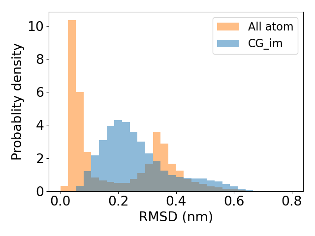
From the above plot, we see that the coarse-grained energy function with just bonded terms reproduces the marginal distribution of every internal coordinate. However, reproducing marginal distributions does not guarantee that the energy function reproduces the conformational ensemble. One way to see that is comparing the distribution of RMSD between data and noise samples, as shown below.